Megabin
3D versus conventional 3D methods
with examples from the Michigan Basin
Norm Cooper,Ê Mustagh Resources Ltd., Calgary, Alberta
Jim Egden, Union Gas Limited, London, Ontario
ABSTRACT
Two 3D programs were recorded in close proximity in Lambton County of the Michigan Basin by Union Gas Limited.Ê The objectives were to image Silurian pinnacle reefs in a cost effective manner.Ê One 3D employed conventional orthogonal techniques while the other employed the "MegaBin" method.Ê
This paper reviews the design and characteristics of each method.Ê The theory of the "MegaBin" method is explained.Ê We briefly compare aspects of design, acquisition and processing.Ê Samples of each survey are shown to demonstrate some differences in image quality and interpretability.Ê Finally, we will summarize the cost effectiveness of each approach.
A Discussion of Ideal Seismic Imaging
The basic principle of reflection
seismic is to generate an acoustic wavefront in the earth.Ê This is usually accomplished by detonating dynamite
charges buried a few meters below the surface or by using a machine that
vibrates and shakes the earth with a controlled signal spanning a significant
frequency range.Ê Once introduced into
the earth, the wavefront will expand spherically according to the acoustic
velocity of the rocks in which it propagates.Ê
Figure 1ÊÊ
Fundamental seismic imaging.
We introduce an acoustic wave into the earth.Ê As it expands and interacts with the earth, it becomes a complex wavefield, portions of which return to the surface during our seismic record.Ê How frequently in time and space we choose to observe this returning wavefield (and how frequently we choose to inject it)
is called wavefield sampling.
Irregularities in the subsurface
will distort the developing wavefield.Ê
Each distinct boundary between rock layers of different types will cause
the wavefront to bifurcate into reflected and transmitted elements.Ê The wavefield becomes complex and is
uniquely determined by the geologic changes within range of the seismic
experiment.Ê We record the wavefield at
the surface where, during the time of our seismic record, portions of the
wavefield return (see Figure 1).Ê Our
seismic record length varies from basin to basin and is usually not much longer
than one second in the Michigan Basin.Ê
The wavefield consists of continuous
changes in time and space.Ê By observing
and recording these changes, we hope to reconstruct an image of the geologic
features which distorted the wavefield to be just the way it is.Ê This reconstruction process is the task of
the data processors and interpreters.Ê
For reasons of economic and equipment limitations, we are not able to
record the wavefield continuously at all points in time and space.Ê The job of the program designers and
acquisition contractors is to ensure that we record a sufficient subset of the
full wavefield so that the processors and interpreters can do their part of the
job.Ê
Historically, we have recorded data
in time at a sample interval of 1, 2 or 4 milliseconds.Ê In the Michigan Basin, the most common
sample rate today is 1 millisecond.Ê
This proves to be sufficient to record the frequencies of the wavefield
that survive during our seismic experiment.Ê
We often find useable data from 10 Hz to 180 Hz.Ê These frequencies should allow us to image
features as small as 15 to 20 meters at the Silurian Guelph level.Ê Therefore, 3D surveys are typically designed
to yield bin sizes (stacked trace intervals) of 15 to 20 meters.Ê This determines the basic spatial sample
interval at the surface of 30 to 40 meters.Ê
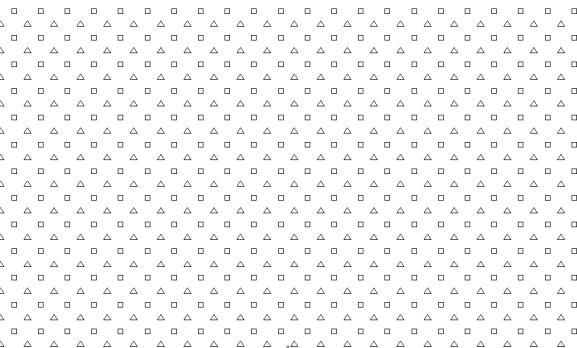
Figure 2ÊÊ
Diagram
of a "Full Wave Field Sampled"
3D layout.
In this example the receivers (triangles) are 40 m apart along each line
and there is a line of receivers every 40 meters.Ê
The sources (squares) are organized in the same pattern but offset from the receivers.
In order to fully sample the
returning wavefield at such a spatial frequency, we should use a grid of
receivers with one trace being generated every 40 meters by 40 meters at the
surface.Ê In order to fully image the
subsurface with sources from all angles and directions, we should use a grid of
source points generating wavefronts every 40 meters by 40 meters.Ê In order to optimize the statistical
diversity of the seismic experiment we should offset the source and receiver
grid.Ê Figure 2 shows such an
arrangement.Ê
For each shot that is generated, we
must record traces within the maximum useful offset as determined by our target
depth and the overlying velocity structure.Ê
For the examples considered in this study, the maximum useable offset
for the Silurian Guelph reefs is about 450 meters.Ê
If we record all of the shots in the
grid described in figure 2 at different times, we will produce overlapping
images of the subsurface which will strengthen the image quality.Ê The amount of overlap is called the
"fold" of the survey.Ê For the
grid in figure 2, we can calculate the fold in each 20 m by 20 m subsurface
bin.Ê This is displayed in figure 3
where we observe the nominal fold to be 100 (except at the edges of the survey
where imaging statistics are deficient).Ê
So each subsurface area of 20 x 20 meters will be imaged by 100 different
traces generated by different source-receiver combinations.Ê What a wonderful level of statistical
sampling · if only we could afford it !
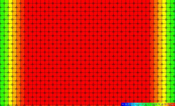
Figure 3ÊÊ
Full Wavefield Sampling ö fold to 450 meter offsets.
The edges of the survey drop below 50 fold, but all bins in the center are 98 fold.
The above discussion details a
design known as "Full Wavefield Sampling".Ê Given spatial and temporal bandwidth limitations, our minimum
realizable sample intervals are defined.Ê
Ideally, we would like to sample our data at these intervals in all
domains.Ê Unfortunately, this would
place high demands on equipment utilisation, landowner impact and program
cost.Ê Let us study two different compromises
to full wavefield sampling.Ê One is
typical of "orthogonal" 3D designs often used in the Michigan Basin,
the other is the "megabin" approach developed by PanCanadian
Petroleums in Alberta.
One Alternative ö The Megabin Design
Let'sÊ examine the impact on the fold if we start decimating the full
wavefield sampled 3D.Ê First, let's
remove every second line of source points in the north-south direction (see
figure 4).Ê Note that the fold drops to
a peak of 50 and the level of fold alternates slightly in north south stripes.Ê This is called "striping" or
"banding" by 3D designers and can be destructive to the image quality
if exaggerated.Ê At this level it is
absolutely no problem as variations are small compared to the median fold.
Ê
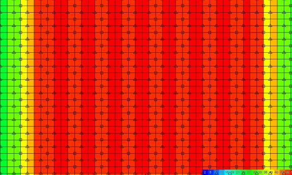
Figure 4ÊÊ
¸ Source Sampling ö fold to 450 meter offsets.
Every second north-south source line has been eliminated.Ê Full fold varies between 47 and 51.
Figure 5 illustrates the results of
further decimation where we have removed every second line of receivers in the
north-south direction.Ê Notice that the
fold in imaged bins remains the same, but now we fail to illuminate every
second column of in-line bins.Ê This is
characteristic of the "megabin" method and does not represent any
significant problem.Ê The greatest
danger is the aliasing of the migration process.Ê Therefore, prior to migration, the data set is interpolated to
fill the missing columns.Ê Generally, a
robust F‑X domain interpolation operator is used (Spitz, 1991 or Porsani,
1999).Ê This provides meaningful trace
data (to the extent that the number of dips does not exceed the number of lines
in the design window).Ê After migration,
both interpolated and original recorded data are mixed and moved within the
migration aperture.ÊÊ Every
post-migration trace consists of a mixture of both original and interpolated
traces.
Figure 6 shows the impact of
deleting one half of the remaining source points.Ê Of course, fold is reduced to a maximum redundancy of 25 traces
per bin and there is still a mild heterogeneity from one column of bins to the
next.Ê This is of no significance
provided the median remains above 10 fold.Ê
Figure 7 is a minor adjustment where the source points are moved from
their staggered position to a location in line with the receivers.ÊÊ This enables the program to be recorded
from a single set of parallel lines and minimizes landowner impact.
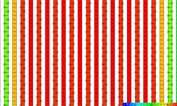
Figure 5ÊÊ
¸ Source ¸ Receiver Sampling ö fold to 450 meter offsets.
Full fold varies between 47 and 51 in imaged bins and zero in alternate bins.
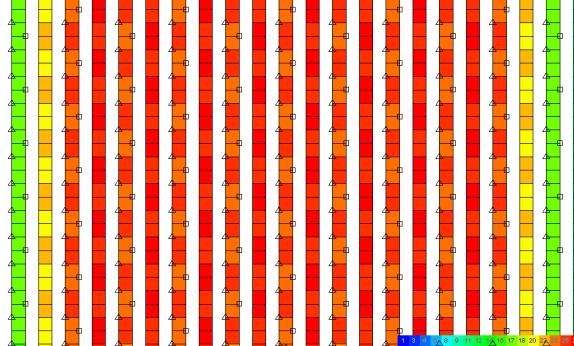
Figure 6ÊÊ
¹ Source ¸ Receiver Sampling ö fold to 450 meter offsets.
Fold is 25 and 26 between surface lines;Ê 23 and 24 below surface lines.
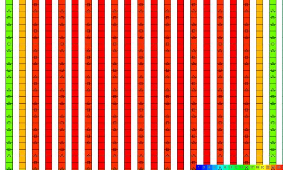
Figure 7ÊÊ
Megabin ö fold to 450 meter offsets.
Fold is 26 between surface lines;Ê 24 and 25 below surface lines.
Figure 7 shows the design developed
by PanCanadian Petroleums known as "megabin".Ê It is one approximation to full wavefield
sampling where only half the required number of receivers are used.Ê This reduces the line density and lowers
landowner impact and survey cost.Ê The
penalty paid in image value is that every second bin in the crossline direction
remains un-imaged.Ê This deficiency is
compensated by applying a spatial interpolation before migration.Ê The sources are sparsely sampled by a factor
of one half in both inline and crossline directions.Ê The effect is to reduce fold in imaged bins and reduce some
offset statistics (to be demonstrated later).Ê
The crossline decimation is necessary to be consistent with the receiver
line decimation and to enable the reduction of line spacing.Ê The inline decimation is not entirely
necessary, but for larger fold 3D's is not significantly detrimental to image
quality and this decimation helps reduce costs (at least in dynamite
surveys).Ê It should be noted that
vibroseis megabin 3D's should still occupy every source point but perhaps use
one half of the expected vertical stack effort (half the number of sweeps).
Note that with sources and receivers
falling on coincident lines, it is not necessary to have orthogonal lines
connecting sources.Ê This savings in
linear kilometers of line to be produced (as well as reduced permitting and
damages) makes the megabin very cost effective in areas where dense grid 3D's
are being considered.
Another Alternative ö the Orthogonal Design
Let's start again with the full
wavefield sampled 3D pictured in figures 2 and 3.Ê Only this time (for consistency with later examples, we will
sample the surface in 30 meter intervals (in both source and receiver
domains).Ê This will yield subsurface
sampling in 15 meter bins.Ê The fold
diagram (again limited to the useful offsets of 450 meters at the Silurian
Guelph level) is shown in figure 8.Ê
This time (due to the tighter grid density), the nominal fold is about
176.

Figure 8ÊÊ
Full Wavefield Sampling ö fold to 450 meter offsets.
The edges of the survey drop below 50 fold, but all bins in the center are 179 fold.
The fold diagram in figure 9 results
when we eliminate two out of three source lines in the east-west
direction.Ê In this decimation, we are
left with east-west lines of source points and the source line spacing is 90
meters.Ê The resulting fold is reduced
to one third (on average) and now appears to vary between 58 and 62.Ê This represents a slight heterogeneity and
shows east-west banding.Ê However, with
the high level of average fold, this will not adversely effect the data.
We further decimate the data in
figure 10 by eliminating half the receivers (every second north-south
line).Ê We now have an orthogonal grid
of data with a 90 meter source line spacing and 60 meter receiver line
spacing.Ê Notice that the orthogonal
arrangement of sources and receivers ensures that every bin will be imaged with
original traces.Ê However, this
decimation reduces fold by a factor of two (now ranging between 28 and 31
fold).Ê We also begin to notice a
checker board pattern of fold variation.Ê
With an average fold near 30, this variation only represents a plus or
minus 6 percent fluctuation and we are not yet concerned about geometric
imprinting in the data.
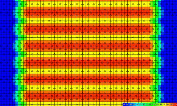
Figure 9ÊÊ
Source 90 Receiver 30 ö fold to 450 meter offsets.
Full fold varies from 58 (between source lines) to 61 (below source lines).
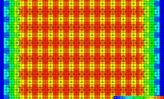
Figure 11 represents one more level
of decimation where we have removed half of the remaining receiver lines to
produce an orthogonal grid with source lines spaced 90 meters apart and
receiver lines spaced 120 meters apart.Ê
The fold now varies from 12 to 16 (14 plus or minus 2).Ê This is a 14 percent variation around the
median fold and, in our experience, may be sufficient to generate a mild amount
of geometric imprinting.Ê
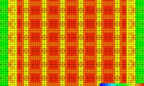
Figure 11ÊÊ
Source 90 Receiver 120 ö fold to 450 meter offsets.
Full fold varies from 13 (below receiver lines) to 16 (darker colors).
Of course, fold is not the most
important statistic to concern ourselves with.Ê
In the following series of figures, we will compare the offset
distribution of an ideal (full wavefield sampled) 3D to the megabin approximation
and the tight grid orthogonal.Ê
Offset distribution plots indicate
the source-receiver offset characteristics of the collection of traces that
image each bin.Ê In figure 12, each bin
is imaged by 176 traces.Ê Some of these
traces were generated by source-receiver pairs in close proximity to each other
(near offsets) and are represented by very short vertical line segments located
at the left of each bin.Ê Long offset
traces are represented by longer vertical line segments positioned at the right
side of each bin.Ê A bin that is imaged
by a broad variety of offsets will appear as a filled triangle.Ê The color (or grey shade) of each vertical
line segment indicates statistical redundancy.Ê
That is, some offset ranges are repeated by more than one trace.Ê Fold generated by statistically diverse
offset distribution is constructive for enhancing signal to noise ratio in the
stack process.Ê Redundant observations
contribute much less value in the stack.Ê
The full wavefield sampled survey
shown in figure 12 has sampled at least one trace in every possible offset
range (n ± ¸Ê
«Ê
bin size in metersÊÊÊ [for n=1 to
30 representing 15 to 450 m of offset]) except for the offset atÊ 2 ±
¸Ê «
15 m.Ê Note that we collect traces in
offset ranges centered on integer multiples (n) of our bin size.Ê Each vertical bar represents one value of
n.Ê The left most (short) bar represents
n=1 or an offset ofÊ 0.5 to 1.5 bin
sizes.Ê The next bar represents 1.5 to
2.5 bin sizes (n=2).Ê The last bar
represents the maximum useable offset (n = Xmax / bin size).
In the middle and far offsets, there
is a high level of redundancy.Ê This is
a result of wide aperture recording where we expect 5/9 of our traces to come
from the far third of the offset range and only 1/9 to come from the near
third.Ê
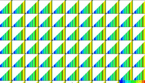
Figure 12ÊÊ
Full Wavefield Sampling ö offset detail.
Redundancy ranges from 0 to 10 observations per offset.
Figure 13 shows the offset
distribution resulting from the megabin model.Ê
Note that the bins between surface lines are quite well imaged, while
the bins underlying the surface lines demonstrate a few offset
deficiencies.Ê Any time we choose not to
record full wavefield sampling, we must sacrifice some of our statistical
sampling.Ê In this model, the patterns
occur in pairs due to the sparse source sampling along the surface lines.Ê These bins would be better sampled and
uniform if the source interval matched the receiver interval (an affordable
strategy for vibroseis programs).Ê
Figure 14 is the offset distribution
resulting from the orthogonal model.Ê
Notice the significant bin to bin heterogeneity.Ê Most bins have significant deficiencies
(large gaps of missing offsets).Ê We
concern ourselves with the "clumpiness" of offset distributions.Ê There are small regions of offsets densely
sampled and other regions very sparsely sampled.Ê The character of this "clumpiness" varies greatly from
one bin to the next.Ê
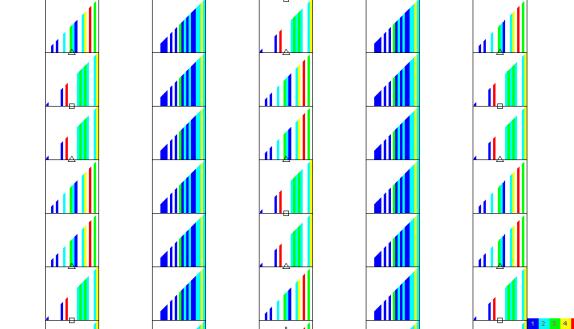
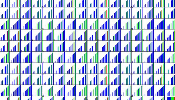
Figure 14ÊÊ
Source 90 Receiver 120 ö offset detail.
Redundancy ranges from 0 to 3 observations per offset.
In order to study the patterns of
"clumpiness" on a larger scale, we have developed a
"homogeneity" plot.Ê Figure 15
shows the offset homogeneity for the full wavefield sampled model.Ê For each bin, we calculate the distribution
of traces as a function of offset squared (to account for wide aperture
recording).Ê We then tabulate the
differences in offset between each successive offset in a sorted list.Ê A bin containing well distributed offsets
will have a small standard deviation in these differences.Ê A "clumpy" distribution will yield
a larger standard deviation.Ê The
standard deviation of the delta-offset-squared list represents a single number
which can be plotted for each bin and represents the uniformity of offset
sampling in each bin.Ê A small standard
deviation is good (less than 4 percent),Ê
values from 4 to 8 represent fair sampling, and values in excess of 8 to
10 percent represent quite poor offset sampling.Ê Full wavefield sampling shows all full-fold bins with about 1
percent standard deviation.Ê This
represents excellent offset statistics.
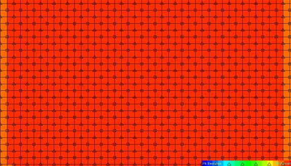
Figure 15ÊÊ
Full Wavefield Sampling ö offset homogeneity.
Standard deviation in full fold bins is 1.34 percent.
Figure 16 is the offset homogeneity
plot for the megabin model.Ê The bins
between surface lines exhibit standard deviations of about 2 percent while the
bins below the surface lines vary in the 5 to 6 percent range.Ê This survey is very well sampled in offset.
Figure 17 is the offset homogeneity
for the orthogonal model.Ê About half
the bins exhibit more than 6 percent standard deviation.Ê This is not very bad by standards for surveys
in the western Canadian basin, but is still substantially inferior to the
megabin model.
Many other statistical measures can
be compared for these two models (largest offset gaps, azimuth distribution,
azimuth homogeneity, largest azimuth gaps).Ê
However, we will reserve these comparisons for the real data examples
that follow.Ê
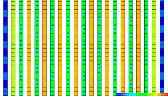
Figure 16ÊÊ
Megabin ö offset homogeneity.
Standard deviation is 2.52 % between surface lines and 5.09 or 5.37 below surface lines.
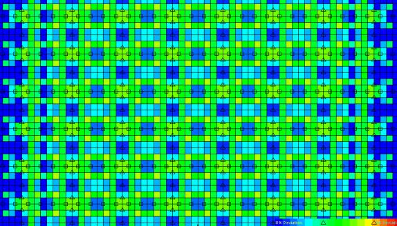
Figure 17ÊÊ
Source 90 Receiver 120 ö offset homogeneity.
Standard deviation in full fold area varies from 3.3 (lighter colors) to 7.41 (darker colors).
Statistical Evaluation of Case Histories
Figure 18 shows the relative
location of two 3D surveys conducted in SW Ontario.Ê The survey to the southeast is known as Bentpath East and was
recorded in September of 1997.Ê The
survey to the northwest is called Booth Creek and was recorded in the summer of
1998.ÊÊ The centers of the two surveys
are less than 2 kilometers apart.
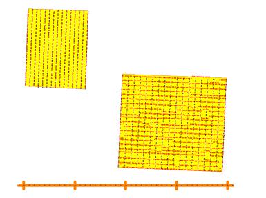
Figure 18ÊÊ
Booth Creek versus Bentpath East ö basic grids and relative location.
Major divisions on scale are separated by 1000 meters.
The following table summarizes
information and parameters for the two surveys:
|
|
Booth Creek |
Bentpath East |
|
Design Consultant |
Mustagh |
Geo-X |
|
Acquisition Contractor |
Can Geo |
Can Geo |
|
Date Acquired |
Summer, 1998 |
September, 1997 |
|
Model Style |
MegaBin |
Orthogonal |
|
Size |
1.530Ê xÊ 1.176Ê km |
2.040Ê xÊ 1.800Ê km |
|
Area |
1.8Ê km2 |
3.67Ê km2 |
|
Recording System |
Das ö 1 ms sample rate |
Das ö 1 ms sample rate |
|
Receiver / SourceÊ Interval |
34 x 68 m |
30 x 30 m |
|
Receiver / Source Line Spacing |
84 x 84 m |
120 x 90 m |
|
Natural Bin Size |
17 x 42 m |
15 x 15 m |
|
Processed Bin Size |
17 x 21 m |
15 x 15 m |
|
Patch (lines and stations) |
12 x 34 (double shot) |
16 x 36 (double shot) |
|
Patch Size |
1008 x 1156 m |
1920 x 1080 m |
|
Receiver Points |
689ÊÊ (383 per km2) |
1098ÊÊ (299 per km2) |
|
Source Points |
338ÊÊ (188 per km2) |
1451ÊÊ (395 per km2) |
|
Linear Receiver / Source km |
22.950 |
32.400 + 42.840 |
|
Linear kms per km2 ö
actual |
12.755 |
20.490 |
|
Linear kms per km2 ö
theoretical |
11.905 |
19.444 |
Figure 19 compares the fold in
natural bins for the two surveys.Ê Note
that the natural bins for Booth Creek are quite large (hence the name
"MegaBin").Ê However, this
data will be gathered in half size bins (as in figure 20), leaving every second
bin empty.Ê A robust F-X domain
interpolator is used to infill the empty bins prior to migration.Ê In figure 19 the fold scales are different
for the two surveys (2-34 and 1-17).Ê In
figure 20 the figures share a common fold scale (13-29).
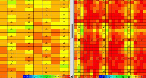
Figure 19ÊÊ
Booth versus Bentpath fold in natural bins.
Booth varies from 24 to 31 fold;Ê Bentpath varies from 11 to 20 fold.

Figure 21 compares the offset
distribution for the two surveys.Ê Note
the greater deficiencies in the orthogonal design.Ê Figure 22 highlights the worst case deficiency (or
"gap") for each bin.Ê The
orthogonal survey varies from 67 to 180 m with a significant number of large
gaps and great variation from bin to bin.Ê
The megabin design is more uniform with most of the gaps from 82 to 119
meters.
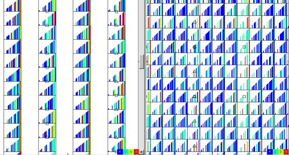
Figure 21ÊÊ
Booth versus Bentpath offset distribution.
Note the bin to bin uniformity of the MegaBin design.
In figure 23 we have presented the
offset homogeneity plot for the two surveys.Ê
Notice that the megabin survey yields much more uniform offset sampling
in all bins.Ê Homogeneous offset
sampling is very important to stacked data quality, the consistency of multiple
suppression and the stability of wavelet phase and amplitude.Ê
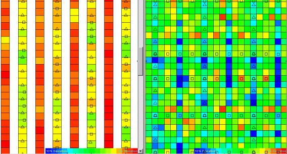
Figure 23ÊÊ
Booth versus Bentpath offset homogeneity.
Booth ranges from 2.3 to 4.7 %;Ê Bentpath ranges from 2.5 to 11.3 % standard deviation.
Another important statistic of
interest to 3D designers and processors is azimuth distribution.Ê Image quality is enhanced if each stacked
trace is the average of observations of the subsurface reflection from many different
angles.Ê Figure 24 shows the
source-receiver alignment for all of the traces contributing to each subsurface
bin.Ê We refer to this as a
"spider" diagram.Ê The length
of each leg of the spider is proportional to the source-receiver offset for
that trace.Ê A well sampled survey will exhibit
bin to bin consistency in the spider plot and each bin will have a spider with
legs of different lengths pointing in all different directions.
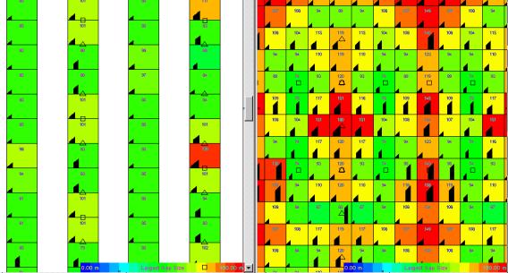
In each bin, we can sort the
contributing traces by azimuth.Ê Then we
calculate the difference in azimuth between adjacent traces.Ê Figure 25 shows a plot of the largest such
angle for each bin.Ê This "largest
azimuth gap" indicates the worst occurrence of deficient azimuths of
imaging for each stacked trace.Ê The
higher fold of the megabin design helps reduce the largest gap in azimuth.Ê The density of the sampling stabilizes the
bin to bin variation.Ê
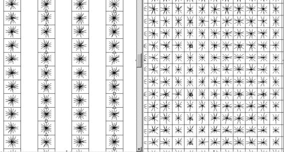
Figure 24ÊÊ
Booth versus Bentpath azimuth distribution.
Note the more consistent appearance of the megabin distribution. Ê
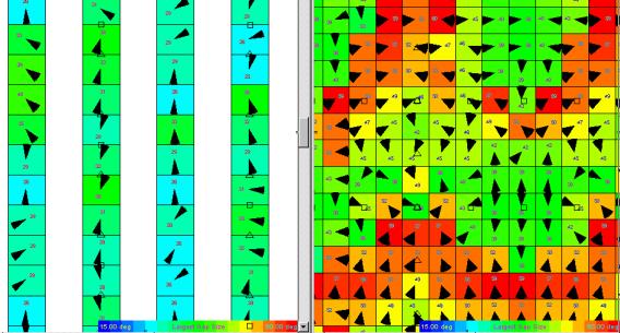
Figure 25ÊÊ
Booth versus Bentpath largest azimuth gap.
The orthogonal design not only has larger gaps, but they are more erratic in azimuth from bin to bin.
Booth varies fromÊ 26 to 40 degrees;Ê Bentpath varies from 38 to 59 degrees.
If we use the same list of
delta-azimuths, we can measure the standard deviation of the distribution for
each bin .Ê This will provide a single
number that can be associated with the azimuth homogeneity of each bin.Ê A low standard deviation means that azimuths
are uniformly sampled.Ê A higher
standard deviation reflects more heterogeneity in azimuth distribution within
each bin.Ê
Figure 26 shows the azimuth
homogeneity for the subject surveys.Ê
Homogeneous values (small values of standard deviation) indicate a
stacked trace resulting from the average of well sampled raypaths.Ê Consistency of color from one bin to the
next indicates stability from trace to trace in the stacked data volume.Ê
Note that the strength of the
standard deviation is not influenced by fold.Ê
In other words, 6 traces well distributed with 60 degrees between each
trace will provide a zero standard deviation the same as 12 traces well
distributed with 30 degrees between each trace.Ê Therefore, the strength observed in the megabin azimuth
homogeneity plot versus the orthogonal version is due to more uniform
statistical sampling.
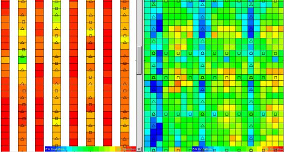
Figure 26ÊÊ
Booth versus Bentpath azimuth homogeneity.
Booth varies from 1.97 to 2.99 % standard deviation;Ê Bentpath from 2.74 to 5.63 % standard deviation.
The accumulation of statistical
analysis weighs heavily in favor of the megabin design.Ê Because both source lines and receiver lines
occupy the same physical line on the ground, the total linear kilometers to be
permitted, produced, surveyed and travelled is less for the megabin versus the
orthogonal.Ê For the two surveys
considered here, the megabin used 62 percent of the linear kilometers per
square kilometer of surface coverage.Ê
The overall costs of the megabin survey (on a per square kilometer
basis) were 20 to 30 percent lower than the orthogonal.Ê
Data Comparison of Case Histories
Figure 27 is a grid map of the
Bentpath East 3D as it was acquired.Ê
Note the extra effort involved in offsetting source segments around
cultural features.Ê Consider the
additional amount of access trail and permit damages to be paid associated with
servicing these offset locations.Ê
Figure 27ÊÊ
Bentpath East Orthogonal 3D grid as it was acquired.
Orthogonal 3D's require careful
skidding and offsetting procedures to bypass cultural obstructions.Ê
This increases landowner costs and damages due to additional access.Ê Offsetting often results in some confusion
in locating shots during recording.
Figures 28 and 29 show time slices
through the processed data volume from the Bentpath survey at 304 ms and 315 ms
respectively.Ê These reveal the crest
and the base of a large reef.Ê The reef
is clearly imaged. The strong linear feature across the south boundary of the
shallow slice is a result of major salt solution associated with the Dawn
fault.Ê
The time slices also illustrate the
location of inline 65 (A-A') and crossline 64 (B-B').Ê These two data slices are reproduced in figures 30 and 31
respectively.Ê Note the clear evidence
of a large reef on these sections.Ê
Note, also the unstable nature of most reflections.Ê See how many of the weak and moderate
reflectors appear to alternate every few traces from stronger to weaker.Ê This lack of consistency of character and
amplitude is a result of a certain amount of geometric imprinting of the
orthogonal geometry and its statistical deficiencies.Ê This phenomenon also casts doubt on some of the character and
amplitude changes observed in the time slices.
This feature was tested by two wells
prior to the recording of the 3D.Ê Since
the interpretation of the 3D, three more wells have been drilled that confirm
the interpretation.
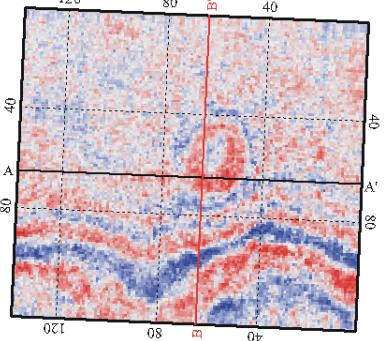
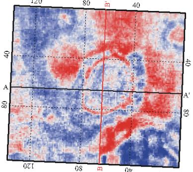
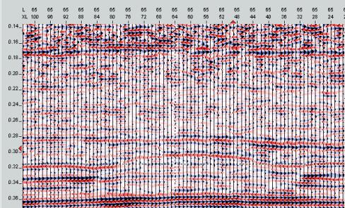
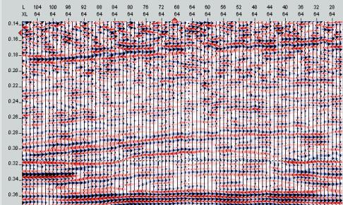
Figure 32 is a detail plot of the
Booth Creek 3D grid as it was acquired.Ê
Notice that some shot points have been missed and others have been made
up along existing lines at unused shot locations.Ê Skidding and offsetting is not a difficult issue in a megabin
design since we have already occupied at least half of the valid source
locations.Ê Usually, our fold is so high
that we are not concerned about maintaining level of fold around gaps.Ê Our greatest concern is to try to maintain
optimal near offset contributions.Ê Any
shots located between existing lines would not compliment coverage in any of
the modelled imaged bins.Ê Therefore,
such shots are not constructive additions to the program and we eliminate any
additional access.Ê
Figure 32ÊÊ
Booth Creek Megabin 3D grid as it was acquired.
Note there is no abnormal access to service make-up shots around cultural obstructions.
Figures 33 to 36 show a series of
time slices from the Booth Creek 3D (356, 353, 348 and 332 ms).Ê The development of a broad, low relief reef
with a pinnacle crest is clearly evident.Ê
Unfortunately, these displays were created from a different work station
with bolder colors and some edge smoothing.Ê
This makes the overall appearance different to the Bentpath time
slices.Ê However, note how small the
Booth Creek pinnacle crest is.Ê Less
than 200 meters across, the rim of this feature contains two lobes, each only
about 50 meters across.ÊÊ Yet the larger
bins of the megabin design (and the interpolated traces) are clearly able to
map this tiny detail.Ê This is a
testament to the image quality and statistical wavefield samplingÊ inherent in the megabin method.Ê
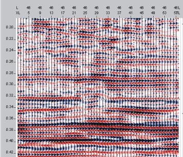
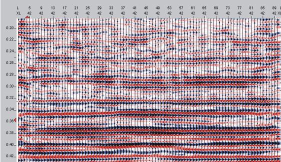
Figures 37 to 39 show some samples
of the data slices through the crest of the reef (inline 46 and crossline 28
intersect over the crest) as well as near the edge of the low reef buildup
(crossline 42).Ê Note the general
consistency of the reflection strength and character even in the shallow events
(280 ms).Ê There is no evidence of
geometric imprinting in this data.Ê
This prospect was tested in the low
reef position by two wells prior to the recording of the 3D.Ê There was no indication of the
pinnacle.Ê Since the interpretation of
the 3D, two more reef crest wells have been drilled.Ê The interpretation has been proven by the drill bit!
Conclusions
The megabin style of 3D was
introduced to SW Ontario in 1998.Ê Since
then, many 3D programs of this style have been recorded.Ê Cost savings of 20 to 30 percentÊ over more conventional 3D programs have been
realized.Ê Landowner impact is greatly
reduced and the task of permitting is made somewhat easier.Ê These benefits alone would justify the
method even if there was a slight deterioration of data quality.Ê The fact is, the megabin technology provides
better sampling statistics than recent conventional designs.Ê The image quality is enhanced and
stabilized.Ê Interpretation is more
reliable than it has ever been.
The megabin strategy works very well
in the Michigan Basin, partly due to the shallow target depth.Ê In much deeper basins, where longer
source-receiver offsets are useful, the bin-driven design of the megabin
becomes more costly compared to sparse, fold-driven designs.ÊÊ The image quality of megabin is the closest
3D equivalent of the 2D "stack array" strategy.Ê It can provide the best wavefield sampling
and deliver statistics valuable to the processor and interpreter.Ê For prospects where long source-receiver
offsets are available, the cost ratio of megabin to conventional design makes
the megabin method difficult to defend.Ê
However, for shallower targets it represents the cheapest, lowest impact
and best image quality of all options to the users of 3D methods.
Acknowledgments
The authors would like to thank
Union Gas Limited for sharing their data sets with the industry to promote
better understanding of modern methods.Ê
They showed the courage and the insight to try new methods.ÊÊ
CanGeo Ltd. provided much input and
helped adapt the megabin method to suit SW Ontario operational
considerations.Ê
We will always be indebted to Bill
Goodway and Brent Ragan of PanCanadian Petroleums who developed and enhanced
the megabin technology.Ê Admirably,
PanCanadian has chosen to openly share this technology with the industry.Ê They have patented the method primarily as a
defensive measure to protect it from patent by others.Ê This gives them the control to keep the
method open to all potential users.Ê
REFERENCES
Goodway, Bill and Ragan, Brent,
Personal Communication
Porsani, Milton J., September-October 1999.Ê Seismic Trace Interpolation Using Half-Step Prediction Filters.Ê Geophysics, volume 64, number 5, pages 1461-1467, Society of Exploration Geophysicists.
Spitz, S., June 1991.ÊÊ Seismic Trace Interpolation in the F-X Domain.Ê Geophysics, volume 56, number 6, pages 785-794, Society of Exploration Geophysicists.